Wikihow Text Summarization
Text Summarization using deep learning
The Purpose of this notebook is to summarize the cleaning, preprocessing and modeling of the Wikihow dataset. For the purpose of making the notebook more concise, many of the cells and code required to develop this project have been excluded. The full code can be found through these links:
Project Intro
Text summarization is the process of taking a larger text and condensing it into the components which elicit the most useful information. While certain techniques such as TF-IDF and Naive Bayes can identify patterns and consistencies, they fail at remembering word order. Because of this, these techniques can’t make use of the context in which the words are said and lose vital information with regard to context. Deep learning models are capable of remembering word placement and can create more comprehensive summaries.
import pandas as pd
import numpy as np
import re
from keras.preprocessing.text import Tokenizer
from keras.preprocessing.sequence import pad_sequences
from nltk.corpus import stopwords
import matplotlib.pyplot as plt
from tensorflow import keras
from tensorflow.keras.layers import Input,LSTM, Embedding, Dense, Attention, Concatenate, TimeDistributed, Masking
from tensorflow.keras.models import Model, load_model
from tensorflow.keras.callbacks import EarlyStopping, ModelCheckpoint
from sklearn.model_selection import train_test_split
from tensorflow.keras.utils import plot_model
import tensorflow as tf
import os
The Data:
The Wikihow dataset was compiled with the purpose of it being used for abstract text summarization. Most text summarization datasets come from news articles, which are written in a style that places the most important facts in the beginning of the text. This makes it easy for summarization models to be out performed by simply taking the first few setences of these texts. The WikiHow dataset is written by regular people and contains procedural steps for completing a task. This means that the text summarization model will have to look for the details throughout the entire text in order to create an accurate summary. The dataset contains three rows: The headline (which will act as the target summary), the article title, and the article text.
# Importing the data
Data = pd.read_csv('Data/wikihowAll.csv')
Data.head()
| headline | title | text | |
|---|---|---|---|
| 0 | \r\nKeep related supplies in the same area.,\r... | How to Be an Organized Artist1 | If you're a photographer, keep all the necess... |
| 1 | \r\nCreate a sketch in the NeoPopRealist manne... | How to Create a Neopoprealist Art Work | See the image for how this drawing develops s... |
| 2 | \r\nGet a bachelor’s degree.,\r\nEnroll in a s... | How to Be a Visual Effects Artist1 | It is possible to become a VFX artist without... |
| 3 | \r\nStart with some experience or interest in ... | How to Become an Art Investor | The best art investors do their research on t... |
| 4 | \r\nKeep your reference materials, sketches, a... | How to Be an Organized Artist2 | As you start planning for a project or work, ... |
Cleaning
In order to prepare this data for training, both the text and headline columns need to be cleaned so that they can be processed by a text tokenizer. In the following cells I perform text processing tasks such as expanding contractions, removing stopwords, and removing unwanted symbols and word endings. I then add these proccessed columns to the dataset as clean versions of their originals.
Data.head()
| headline | title | text | clean_text | cleaned_headline | |
|---|---|---|---|---|---|
| 0 | \r\nKeep related supplies in the same area.,\r... | How to Be an Organized Artist1 | If you're a photographer, keep all the necess... | photographer keep necessary lens cords batteri... | _START_ keep related supplies in the same area... |
| 1 | \r\nCreate a sketch in the NeoPopRealist manne... | How to Create a Neopoprealist Art Work | See the image for how this drawing develops s... | see image drawing develops step step however i... | _START_ create sketch in the neopoprealist man... |
| 2 | \r\nGet a bachelor’s degree.,\r\nEnroll in a s... | How to Be a Visual Effects Artist1 | It is possible to become a VFX artist without... | possible become vfx artist without college deg... | _START_ get bachelor degree enroll in studio b... |
| 3 | \r\nStart with some experience or interest in ... | How to Become an Art Investor | The best art investors do their research on t... | best art investors research pieces art buy som... | _START_ start with some experience or interest... |
| 4 | \r\nKeep your reference materials, sketches, a... | How to Be an Organized Artist2 | As you start planning for a project or work, ... | start planning project work likely gathering s... | _START_ keep your reference materials sketches... |
EDA
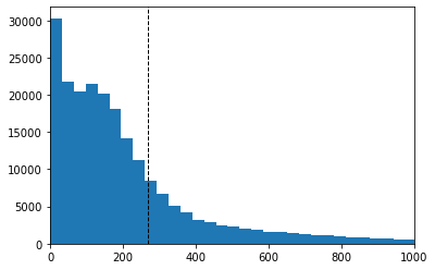
In order to choose the maximum sequence lengths for the models, I create histograms representing the various lengths of each text and headline. Larger sequences lengths can capture more information for inference but make the model take more time to process. The max length has to be set a one value for each of the texts for the model to run. Any text that has a smaller sequence length than the max length will be padded with zeros which will provide no further information but increase processing time. Texts with lengths above the sequence length won’t include texts above the length and that information will be lost. Therefore the optimal sequence length will balance these issues.
np.mean(text_word_count)
219.8083334111081
plt.hist(text_word_count, bins = 200)
plt.xlim(0,1000)
plt.axvline(np.quantile(text_word_count,.75), color='k', linestyle='dashed', linewidth=1)
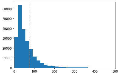
plt.hist(headline_word_count, bins = 200)
plt.xlim(0,500)
plt.axvline(np.quantile(headline_word_count, .75), color='k', linestyle='dashed', linewidth=1)
max_len_text = int(np.quantile(text_word_count, .75))
max_len_headline = int(np.quantile(headline_word_count, .75))
print(max_len_text)
print(max_len_headline)
270
74
The data here shows that 75 percentile for texts are at 270 and 74 for the texts and headlines respectively. Based on this I will round up to 300 and 80 when creating the model. The next step is to preprocess and develop the model so that it can be trained and validated.
Preprocessing and Modeling
Having cleaned and explored the wikikhow test data I will begin preprocessing the data for modeling, building the model architecture, training the model, and finally assessing model performance.
Data = pd.read_csv('Data/Wikihow_clean')
Data = Data.dropna(axis = 0)
Data.head()
| Unnamed: 0 | headline | title | text | clean_text | cleaned_headline | |
|---|---|---|---|---|---|---|
| 0 | 0 | \r\nKeep related supplies in the same area.,\r... | How to Be an Organized Artist1 | If you're a photographer, keep all the necess... | photographer keep necessary lens cords batteri... | _START_ keep related supplies in the same area... |
| 1 | 1 | \r\nCreate a sketch in the NeoPopRealist manne... | How to Create a Neopoprealist Art Work | See the image for how this drawing develops s... | see image drawing develops step step however i... | _START_ create sketch in the neopoprealist man... |
| 2 | 2 | \r\nGet a bachelor’s degree.,\r\nEnroll in a s... | How to Be a Visual Effects Artist1 | It is possible to become a VFX artist without... | possible become vfx artist without college deg... | _START_ get bachelor degree enroll in studio b... |
| 3 | 3 | \r\nStart with some experience or interest in ... | How to Become an Art Investor | The best art investors do their research on t... | best art investors research pieces art buy som... | _START_ start with some experience or interest... |
| 4 | 4 | \r\nKeep your reference materials, sketches, a... | How to Be an Organized Artist2 | As you start planning for a project or work, ... | start planning project work likely gathering s... | _START_ keep your reference materials sketches... |
len(Data)
208885
Preprocessing
Preprocessing the data involves splitting the data into training and test sets. I’ll take eighty percent of the data for training and the rest for validation. After the data is split I initialize values for maximum text length and maximum summary length. I then tokenize the training and validation sets transforming each entry from a readable text to equally lengthed sequences of numbers that can be processed by a word embedding layer. This is done to both the texts and summaries with their respective lengths applied to both the training and test sets
X_train, X_test, y_train, y_test = train_test_split(Data['clean_text'], Data['cleaned_headline'], test_size = .2, random_state = 4, shuffle = True)
print(len(X_train), len(X_test))
167108 41777
# max_len values set the maximum length for both the text and summary these values cames from previous Explorartory Data Analysis
max_len_text = 300
max_len_summary = 80
# The tokenizer creates a 'token' for each word which is a number that corresponds with that word
X_tokenizer = Tokenizer(filters = '!"#$%&()*+,-./:;<=>?@[\\]^`{|}~\t\n', lower = False)
X_tokenizer.fit_on_texts(list(X_train))

# Transforming the sequence of words into a corresponding sequence of their respective tokens
X_train = X_tokenizer.texts_to_sequences(X_train)
X_test = X_tokenizer.texts_to_sequences(X_test)

# Padding ensures that the sequences are all of the same size by adding empty tokens up to the max length
X_train = pad_sequences(X_train,  maxlen=max_len_text, padding='post')
X_test = pad_sequences(X_test, maxlen=max_len_text, padding='post')

# X_tokenizer.word_index['UNK'] = 0
# X_tokenizer.index_word[0] = 'UNK'

x_voc_size = len(X_tokenizer.word_index) +1
y_tokenizer = Tokenizer(filters = '!"#$%&()*+,-./:;<=>?@[\\]^`{|}~\t\n', lower = False)
y_tokenizer.fit_on_texts(list(y_train))


y_train = y_tokenizer.texts_to_sequences(y_train)
y_test = y_tokenizer.texts_to_sequences(y_test)

y_train = pad_sequences(y_train,  maxlen=max_len_summary, padding='post')
y_test = pad_sequences(y_test, maxlen=max_len_summary, padding='post')

# y_tokenizer.word_index['UNK'] = 0
# y_tokenizer.index_word[0] = 'UNK'

y_voc_size = len(y_tokenizer.word_index) +1
# Theses dictionairies can be used to tranform words into tokens or return tokens back to words
reverse_target_word = y_tokenizer.index_word
reverse_input_word = X_tokenizer.index_word
target_word_index = y_tokenizer.word_index
print(x_voc_size, y_voc_size)
140540 67947
Embedding Layer
Rather than having my model develop it’s own word embeddings, This model will use pre trained embeddings from the Word2Vec model. This will save time during training at the sacrifice of certain words not present in the Word2Vec vocabulary not having their own embeddings.
import smart_open
smart_open.open = smart_open.smart_open
from gensim.models import Word2Vec
import gensim.downloader as api
v2w_model = api.load('word2vec-google-news-300')
C:\Users\Allen\anaconda3\lib\site-packages\smart_open\smart_open_lib.py:253: UserWarning: This function is deprecated, use smart_open.open instead. See the migration notes for details: https://github.com/RaRe-Technologies/smart_open/blob/master/README.rst#migrating-to-the-new-open-function
  'See the migration notes for details: %s' % _MIGRATION_NOTES_URL
embedding_matrix_X = np.zeros((x_voc_size, 300))
for word, index in X_tokenizer.word_index.items():
    if word not in v2w_model:
        continue
    else: embedding_matrix_X[index] = v2w_model[word]
embedding_matrix_y = np.zeros((y_voc_size, 300))
for word, index in y_tokenizer.word_index.items():
    if word not in v2w_model:
        continue
    else: embedding_matrix_y[index] = v2w_model[word]
Embedding words not in pretrained embedding
Xemb_trained = []
Xemb_untrained = []
for word, index in X_tokenizer.word_index.items():
    if word not in v2w_model:
        Xemb_untrained.append(word)
    else: Xemb_trained.append(word)
# Percentage of unembedded words in vocabulary
print(len(Xemb_untrained) / (len(Xemb_untrained) + len(Xemb_trained)))
0.4374301795231217
Creating lagged Y’s
In order for the model to be properly trained. The Y variable needs to be lagged by one token so that the data is trained to predict the next word.
y_train_l = y_train.reshape(y_train.shape[0], y_train.shape[1], 1)[:,1:]
y_test_l = y_test.reshape(y_test.shape[0], y_test.shape[1], 1)[:,1:]

end_array_train = np.full((y_train.shape[0],1,1), 0)
end_array_test = np.full((y_test.shape[0],1,1), 0)

y_train_l = np.append(y_train_l, end_array_train, axis = 1)
y_test_l = np.append(y_test_l, end_array_test, axis = 1)

# print(y_train[0,:], y_train_l[0,:])
y_train_l.shape
(167108, 80, 1)
Building the Model
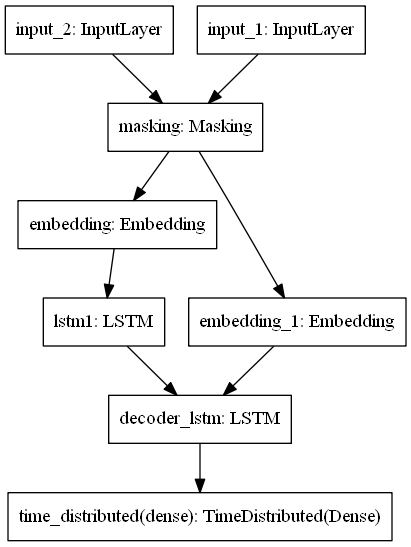
With the data ready to be modeled I use functional Keras to begin constructing an architecture that can model the data. I set the latent dimension which fits the size of the word embeddings and begin with an input that fits the set shape of each text entry. Following the initial input the subsequent layers are input below each designed to receive an input in the shape of its preceding layer. The model is made up of both an encoder and decoer. Encoder part of the model processes the article texts and has a masking layer to ignore padded zeroes, an embedding layer to transform the tokens into their respective embeddings, and a single LSTM layer which produces learned weights from processing the sequences of embeddings. The decoder has a similar structure as the decoder but is designed for the text summary. The decoder’s lstm layer uses the weights learned from the encoder to decide an output. This output is put through a dense layer which returns a probability distribution of possible tokens to predict. If trained well, a sequence of these final tokens should produce a comprehensible summary. The code used to build and train the first model can be seen below along with a model summary and diagram..
from tensorflow.keras import backend as K

K.clear_session()

# The latent dimension is the number of dimensions that each word embedding will correspond with
latent_dim = 300


#Embedding layer
Encoder_inputs = Input(shape=(max_len_text,))

mask = Masking(mask_value = 0)

encoder_mask = mask(Encoder_inputs)


Encoder_embedding = Embedding(x_voc_size, latent_dim,weights = [embedding_matrix_X],trainable=False)(encoder_mask)


lstm1 = LSTM(latent_dim,return_sequences=True,return_state=True, name = 'lstm1')

encoder_output1, h_state, c_state = lstm1(Encoder_embedding)

# Decoder

decoder_inputs = Input(shape=(None,))

decoder_mask = mask(decoder_inputs)

decoder_embedding = Embedding(y_voc_size, latent_dim,weights = [embedding_matrix_y],trainable=False)

dec_emb = decoder_embedding(decoder_mask)


#LSTM using encoder_states as initial state
decoder_lstm = LSTM(latent_dim, return_sequences=True, return_state=True, name = 'decoder_lstm')
decoder_lstm_outputs,decoder_fwd_state, decoder_back_state = decoder_lstm(dec_emb,initial_state=[h_state, c_state])


#Dense layer
decoder_dense = TimeDistributed(Dense(y_voc_size, activation='softmax'))
decoder_outputs = decoder_dense(decoder_lstm_outputs)

# Define the model
model_1 = Model([Encoder_inputs, decoder_inputs], decoder_outputs)
model_1.summary()
Model: "model"
__________________________________________________________________________________________________
Layer (type)                    Output Shape         Param #     Connected to
==================================================================================================
input_2 (InputLayer)            [(None, None)]       0
__________________________________________________________________________________________________
input_1 (InputLayer)            [(None, 300)]        0
__________________________________________________________________________________________________
masking (Masking)               multiple             0           input_1[0][0]
                                                                 input_2[0][0]
__________________________________________________________________________________________________
embedding (Embedding)           (None, 300, 300)     42162000    masking[0][0]
__________________________________________________________________________________________________
embedding_1 (Embedding)         (None, None, 300)    20384100    masking[1][0]
__________________________________________________________________________________________________
lstm1 (LSTM)                    [(None, 300, 300), ( 721200      embedding[0][0]
__________________________________________________________________________________________________
decoder_lstm (LSTM)             [(None, None, 300),  721200      embedding_1[0][0]
                                                                 lstm1[0][1]
                                                                 lstm1[0][2]
__________________________________________________________________________________________________
time_distributed (TimeDistribut (None, None, 67947)  20452047    decoder_lstm[0][0]
==================================================================================================
Total params: 84,440,547
Trainable params: 21,894,447
Non-trainable params: 62,546,100
__________________________________________________________________________________________________
plot_model(model_1)
The following code is used to compile and train the model. Once the model is trained the weights are saved. These saved weights can be used by an encoder and decoder model which reflect the same architecture of the original but are split into their respective parts. Using these models a function can be created to along with the token indices in order to see what the trained model produces from a single input.
es = EarlyStopping(monitor='val_loss', mode='min', patience = 2, verbose=1)
cp_callback1 = ModelCheckpoint(filepath = 'LSTM1_model_train/cp.ckpt', save_best_only = True, verbose  = 1)

model_1.compile(optimizer='rmsprop', loss='sparse_categorical_crossentropy')

history = model_1.fit([X_train,y_train], y_train_l,
                    epochs = 3, batch_size = 50,
                    validation_data = ([X_test,y_test], y_test_l), callbacks = [es, cp_callback1])
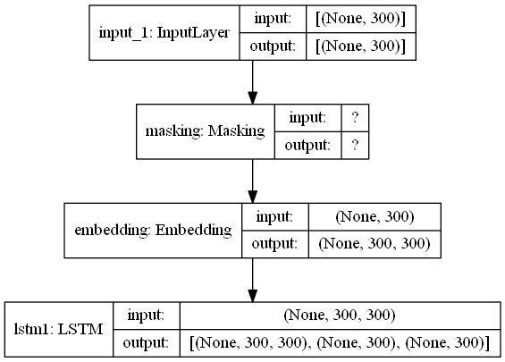
encoder_model1 = Model(inputs = Encoder_inputs, outputs = [encoder_output1, h_state, c_state])
decoder_h_state_input = Input(shape=(latent_dim,))
decoder_c_state_input = Input(shape=(latent_dim,))
decoder_hidden_state_input = Input(shape=(max_len_text,latent_dim))
dec_emb2 = decoder_embedding(decoder_inputs)
decoder_outputs2 , h_state2, c_state2 = decoder_lstm(dec_emb2,initial_state=[decoder_h_state_input, decoder_c_state_input])
decoder_outputs2 = decoder_dense(decoder_outputs2)
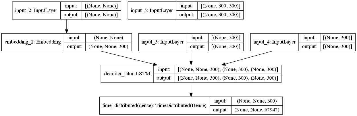
decoder_model1 = Model([decoder_inputs] + [decoder_hidden_state_input, decoder_h_state_input, decoder_c_state_input],
[decoder_outputs2] + [h_state2, c_state2])
plot_model(encoder_model1, show_shapes = True)
plot_model(decoder_model1, show_shapes = True)
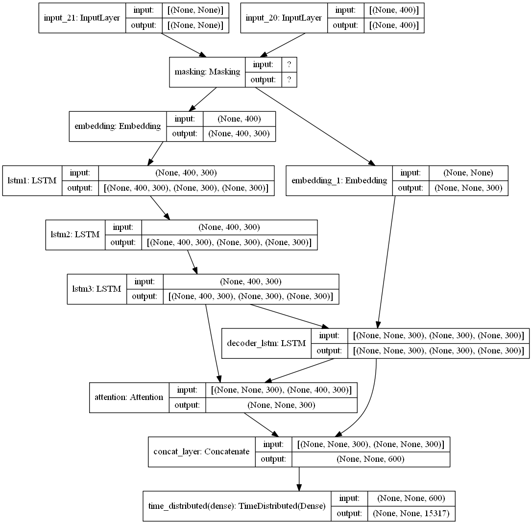
Adding Layers and Attention
I create a more complex model with two additional LSTM layers and an attention layer. The code was more or less the same
plot_model(model2, show_shapes = True,expand_nested = True )
Assessing Performance
results1 = pd.read_csv('Data/model1_training_data.csv')
results1 = results1.drop('Unnamed: 0', axis = 1)
print(results1)
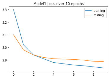
plt.figure()
results1['training'].plot()
results1['testing'].plot()
plt.title('Model1 Loss over 10 epochs')
plt.legend()
   epoch  training  testing
0      1    3.3000   3.1000
1      2    3.0200   2.9800
2      3    2.9400   2.9400
3      4    2.9100   2.9200
4      5    2.8800   2.9100
5      6    2.8700   2.9070
6      7    2.8600   2.9040
7      8    2.8542   2.8992
8      9    2.8454   2.8893
9     10    2.8368   2.8874


<matplotlib.legend.Legend at 0x1d09e5153c8>
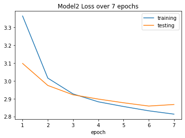
results2 = pd.read_csv('Data/model2_training_data.csv')
results2 = results2.set_index('epoch')
print(results2)
plt.figure()
results2['training'].plot()
results2['testing'].plot()
plt.title('Model2 Loss over 7 epochs')
plt.legend()
       training  testing
epoch
1        3.3646  3.09800
2        3.0155  2.97430
3        2.9267  2.92179
4        2.8824  2.89777
5        2.8560  2.87700
6        2.8318  2.85850
7        2.8131  2.86720


<matplotlib.legend.Legend at 0x1abc46382c8>
Conclusion and Next Steps
At this stage, the model still is extracting very little information from the inputs. Although time consuming, more epochs could be run to continually gain more information during validation. Different layers such as Attention, Bidirectionallayers, and using the Beam search method for decoding could produce better results.